
Optimisation of viewing configurations for 3d-PDV systems
Introduction
It is not possible to measure directly the three orthogonal components of velocity, as there is no practical arrangement of three views, using a single light sheet, where the sensitivity vectors are orthogonal. Therefore, the three measured velocity components must be transformed from the measurement coordinate system (non-orthogonal) to an orthogonal coordinate system. The condition number of the transformation matrix used for this conversion can provide a measure of the suitability of a viewing configuration. A well-conditioned transformation to orthogonal velocity components can be achieved by placing views so that they are well spread and ideally located on both sides of the light sheet. Other factors also have an influence on the performance of a viewing configuration.
- Obstructions in the field-of-view
- Increased light scattering in forward directions leading to better signal levels and hence improved signal-to-noise ratios.
- Forward scattering views will have increased uncertainty due to determining the angle between the view and illumination vectors and in how the Doppler shift uncertainty propagates to velocity uncertainty.
In this work we investigated the optimisation of 3d-PDV viewing configurations and the use of redundant data (by measuring extra velocity components to the three required) to improve the transformation. Extra velocity components can easily be measured using the imaging fibre bundle approach. The following sections give equations for the calculation of the orthogonal velocity components using 3 or 4 measured velocity components.
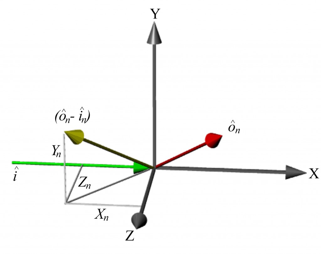
Figure 1 Definitions used in the conversion from measured velocity components to the orthogonal components. Here ôn is the observation direction of the nth view and î is the laser illumination direction; Xn, Yn and Zn are the Cartesian components of the measured velocity (ôn -î) component.
Conversion to orthogonal velocity components – 3C
Using the definitions shown in figure 1 the velocity components can be converted to the orthogonal velocity components, U, V and W using the following expressions given by Reinath[1]
$$U=\frac {1}{Det\left(\left[a\right]\right)}\left[\left|{U}_{1}\right|\left({Y}_{2}{Z}_{3}-{Y}_{3}{Z}_{2}\right) -\left|{U}_{2}\right|\left({Y}_{1}{Z}_{3}-{Y}_{3}{Z}_{1}\right)+\left|{U}_{3}\right|\left({Y}_{1}{Z}_{2}-{Y}_{2}{Z}_{1}\right)\right]$$
$$V=\frac {1}{Det\left(\left[a\right]\right)}\left[\left|{-U}_{1}\right|\left({X}_{2}{Z}_{3}-{X}_{3}{Z}_{2}\right) +\left|{U}_{2}\right|\left({X}_{1}{Z}_{3}-{X}_{3}{Z}_{1}\right)-\left|{U}_{3}\right|\left({X}_{1}{Z}_{2}-{X}_{2}{Z}_{1}\right)\right]$$
$$W=\frac {1}{Det\left(\left[a\right]\right)}\left[\left|{U}_{1}\right|\left({X}_{2}{Y}_{3}-{X}_{3}{Y}_{2}\right) -\left|{U}_{2}\right|\left({X}_{1}{Y}_{3}-{X}_{3}{Y}_{1}\right)+\left|{U}_{3}\right|\left({X}_{1}{Y}_{2}-{X}_{2}{Y}_{1}\right)\right]$$
where
$$\left|{U}_{1}\right|$$, $$\left|{U}_{2}\right|$$, $$\left|{U}_{3}\right|$$ Magnitude of the measured component from camera views 1, 2, and 3.
$$({X}_{1}, {Y}_{1}, {Z}_{1})$$, $$({X}_{2}, {Y}_{2}, {Z}_{2})$$, $$({X}_{3}, {Y}_{3}, {Z}_{3})$$ Unit vector components defining the direction of (ô1-3 – î).
$$U, V, W$$ Orthogonal velocity components, horizontal, vertical and out-of-plane respectively.
Det[(a)] = $${X}_{1}{Y}_{2}{Z}_{3}+ {Y}_{1}{Z}_{2}{X}_{3}+ {Z}_{1}{X}_{2}{Y}_{3}- {Z}_{1}{Y}_{2}{X}_{3}- {X}_{1}{Z}_{2}{Y}_{3}- {Y}_{1}{X}_{2}{Z}_{3}$$
Conversion to orthogonal velocity components – 4C
Extra velocity components can be used in the calculation by using a least square approach where the velocity components can be calculated using the following equations[2]
$$!U=L\left[\left(df-ee\right)g+\left(ce-bf\right)h+\left(be-cd\right)j\right]$$
$$!V=L\left[\left(ce-bf\right)g+\left(af-cc\right)h+\left(bc-ae\right)j\right]$$
$$!W=L\left[\left(be-cd\right)g+\left(bc-ae\right)h+\left(ad-bb\right)j\right]$$
where
$$a=\sum_{i}^{}{{X}_{i}^{2}}{w}_{i}$$ $$b=\sum_{i}^{}{{X}_{i}{Y}_{i}}{w}_{i}$$ $$c=\sum_{i}^{}{{X}_{i}{Z}_{i}}{w}_{i}$$
$$d=\sum_{i}^{}{{Y}_{i}^{2}}{w}_{i}$$ $$e=\sum_{i}^{}{{Y}_{i}{Z}_{i}}{w}_{i}$$ $$f=\sum_{i}^{}{{Z}_{i}^{2}}{w}_{i}$$
$$g=\sum_{i}^{}{{X}_{i}{U}_{i}}{w}_{i}$$ $$h=\sum_{i}^{}{{Y}_{i}{U}_{i}}{w}_{i}$$ $$j=\sum_{i}^{}{{Z}_{i}{U}_{i}}{w}_{i}$$
$$L=\frac{1}{a\left(df-ee\right)-b\left(bf-ce\right)+c\left(be-dc\right)}$$
In these equations the w is the weighting to apply to the measured velocity component, for the simplest case where all views are weighted equally w=1.
Error propagation model
To investigate the selection of viewing configurations a model a 3d-PDV system was written in Matlab[2]. The basic stages of the model are shown in Figure 2.
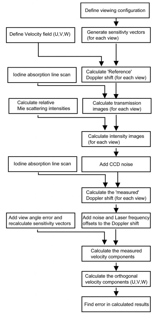 Figure 2 Flow diagram showing the modelling process.
Results
Figure 3 shows modelled results for two configurations compared with experimental results for the same viewing configurations when used to measure the velocity field of a rotating disc.
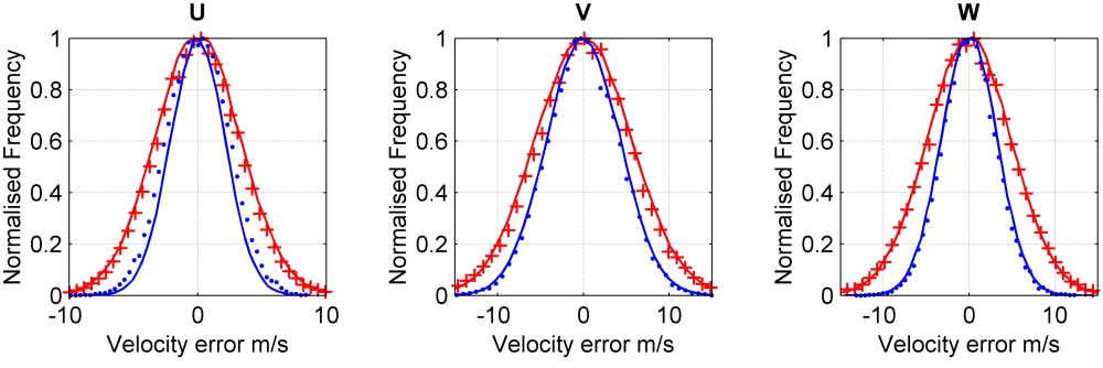 Figure 3 Histograms of the error in the orthogonal components for configuration A (red) and configuration B (blue) for both the simulated (solid line) and experimental results (data points) for the velocity field of a rotating disc.
Figure 4 shows modelled results showing the effect of using extra velocity components in the calculation of the orthogonal velocity components where the 4c significantly reduces the error in two of the three components.
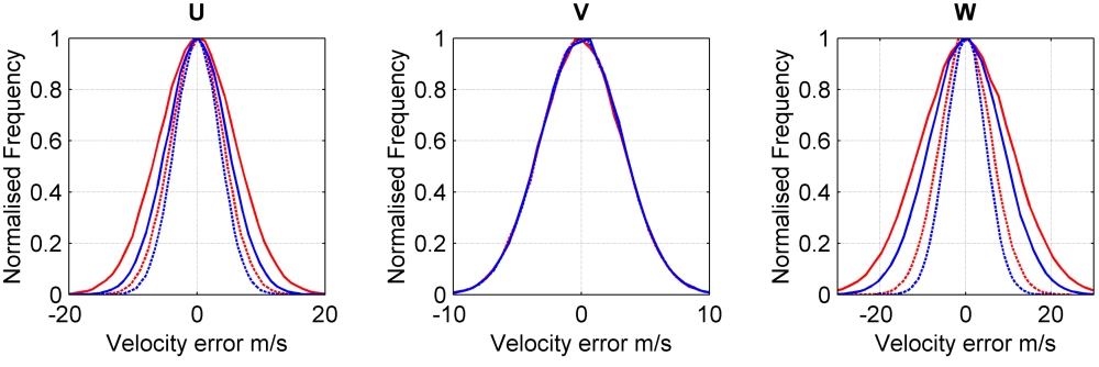 Figure 4 Histograms of error in orthogonal components for configuration A (red) and configuration B (blue). Solid lines show the error using the 3C method of calculating the orthogonal velocity components and the dashed lines show the error using the 4C method.
References
[1] Doppler Global Velocimeter Development for the Large Wind Tunnels at Ames Research Centre.
M.S. Reinath,
NASA , Technical Memorandum 112210, (1997).
[2] Investigation into the selection of viewing configurations for three component planar Doppler velocimetry (PDV) measurements.
Charrett, T.O.H., Nobes, D.S., and Tatam, R.P
Applied Optics. 46, 19, pp 4102-4116. 2007.
[3] Development of two-frequency Planar Doppler Velocimetry instrumentation
Charrett, T.O.H.
PhD thesis, School of Engineering, Cranfield University, 2006